笔记：机器学习的基本工具

本文介绍机器学习的基本 Python 工具和流程。所用算法包括决策树（Decision Tree）、随机森林（Random Forest）和 XGBoost。

基于 Kaggle 教程 Intro to Machine Learning 和 Intermediate Machine Learning。

预备知识

变量的类型

Categorical：人为定义的类别
- Ordinal：有序类别（e.g. Size: S < M < L）
- Nominal：无序类别（e.g. Color: Red, Green, Blue）
Numerical：测量值
- Discrete：离散取值，一般为整数
- Continuous：连续取值

Pandas

参考 Pandas 的常用操作这篇笔记。

预处理

令完整数据集为 home_data，我们将其按 80:20 的比例分为 train 和 validation 两部分。test 数据集为 test_data。

令输入特征为 features，目标变量为 y。

from sklearn.model_selection import train_test_split

home_data = pd.read_csv('data/train.csv')

features = ['LotArea', 'YearBuilt', '1stFlrSF', '2ndFlrSF', 'FullBath', 'BedroomAbvGr', 'TotRmsAbvGrd']
X = home_data[features]
y = home_data.SalePrice

train_X, val_X, train_y, val_y = train_test_split(X, y, random_state=0)

指定 random_state 会使结果可复现。

决策树 & 随机森林

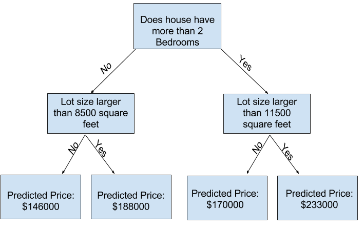
决策树：将样本根据特征 (e.g. LotArea >= 11500 vs LotArea < 11500) 分为两类，然后递归划分所有子集，直到深度达到阈值，或者每个叶子节点的样本数都小于阈值。将每个子集中所有样本的 y 的平均值作为预测值。

伪代码：

def decision_tree(X, y):
    if stopping_condition(X, y):
        return leaf_value(y)
    else:
        split_feature, split_value = find_best_split(X, y)
        X_left, y_left, X_right, y_right = split(X, y, split_feature, split_value)
        return {
            'split_feature': split_feature,
            'split_value': split_value,
            'left': decision_tree(X_left, y_left),
            'right': decision_tree(X_right, y_right)
        }

随机森林：建立多个决策树，每个决策树都是随机生成的。最终预测值为所有决策树的平均值。

from sklearn.tree import DecisionTreeRegressor
from sklearn.ensemble import RandomForestRegressor
from sklearn.metrics import mean_absolute_error

def get_mae(model, train_X, val_X, train_y, val_y):
    model.fit(train_X, train_y)
    preds_val = model.predict(val_X)
    return mean_absolute_error(val_y, preds_val)

# Decision Tree
dt_model = DecisionTreeRegressor()
print(get_mae(dt_model, train_X, val_X, train_y, val_y))

# Random Forest
rf_model = RandomForestRegressor(n_estimators=100)
print(get_mae(rf_model, train_X, val_X, train_y, val_y))

MAE (Mean Absolute Error): $MAE(y, \hat{y}) = \frac{1}{n} \sum_{i=1}^{n} |y_i - \hat{y}_i|$ $M A E (y, \overset{y}{^}) = \frac{1}{n} \sum_{i = 1}^{n} ∣ y_{i} - \overset{y}{^}_{i} ∣$
- mean_absolute_error(y_true, y_pred)
RMSE (Root Mean Squared Error): $RMSE(y, \hat{y}) = \sqrt{\frac{1}{n} \sum_{i=1}^{n} (y_i - \hat{y}_i)^2}$ $RMSE (y, \overset{y}{^}) = \frac{1}{n} \sum_{i = 1}^{n} (y_{i} - \overset{y}{^}_{i})^{2}$
- sqrt(mean_squared_error(y_true, y_pred))

过拟合 & 欠拟合

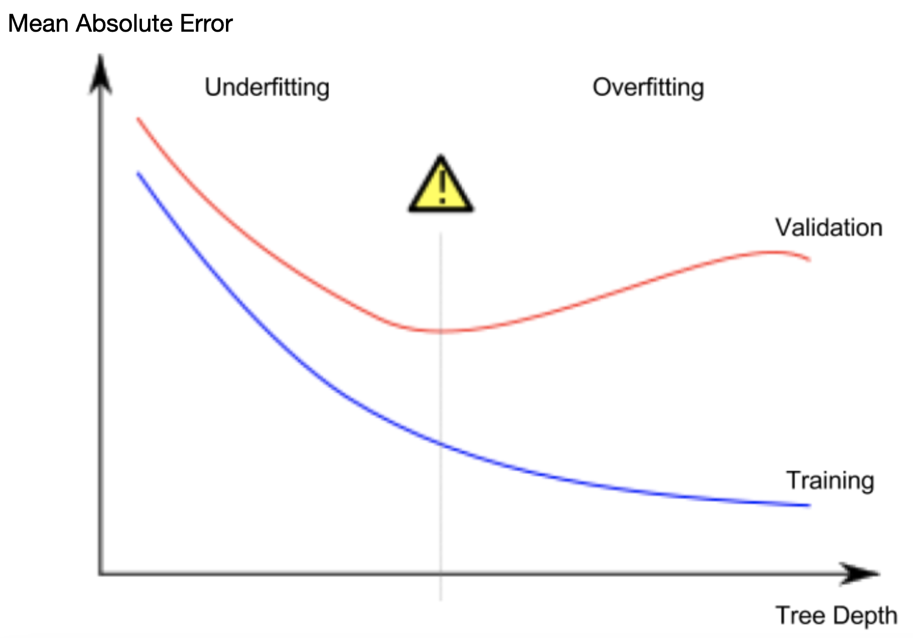
绘制 MAE(train) 和 MAE(validation) 随模型复杂度的变化图，可以看出模型的过拟合和欠拟合情况。

预期情况：MAE(train) 和 MAE(validation) 都下降，但 MAE(validation) 下降速度变慢。
过拟合：MAE(train) 下降，MAE(validation) 上升，表示模型受到训练数据中的噪声影响。
欠拟合：MAE(train) 和 MAE(validation) 都很高。

在决策树中，模型复杂度受 max_leaf_nodes 和 max_depth 制约。（只能设置其中一个）

在随机森林中，n_estimators 越大，模型复杂度越高。

常用参数

n_estimators：决策树的数量
criterion：划分特征的标准
- 默认 squared_error (MSE)，用叶子结点的平均值作为预测值，最小化 L2 loss
- 可选 absolute_error (MAE)，用叶子结点的中位数作为预测值，最小化 L1 loss
max_depth：决策树的最大深度
max_leaf_nodes：叶子结点的最大数量
min_samples_split：如果一个结点的样本数小于该值，则不再划分（默认值为 2）
splitter：划分特征的策略（默认值为 best，即选择最佳划分；可选 random）
max_features：每次划分时考虑的特征数量（默认值等于 n_features，即考虑所有特征）

数据处理

缺失值

选出有缺失值的列：

1 2	missing_val_count_by_column = (X_train.isnull().sum()) print(missing_val_count_by_column[missing_val_count_by_column > 0])

处理缺失值：

(1) 删除有缺失值的列：

cols_with_missing = [col for col in X_train.columns if X_train[col].isnull().any()]

reduced_X_train = X_train.drop(cols_with_missing, axis=1) # axis=1 表示删除列
reduced_X_valid = X_valid.drop(cols_with_missing, axis=1)

(2) 填充缺失值：

from sklearn.impute import SimpleImputer

imputer = SimpleImputer(
    strategy='mean', # 可选 'median', 'most_frequent', 'constant'
    # fill_value=0, # strategy='constant' 时使用
)

imputed_X_train = pd.DataFrame(imputer.fit_transform(X_train))
imputed_X_valid = pd.DataFrame(imputer.transform(X_valid))

# 恢复列名
imputed_X_train.columns = X_train.columns
imputed_X_valid.columns = X_valid.columns

注意 strategy 的选择：ordinal 变量可能不适合用均值填充。（e.g. YearBuilt 应该用 most_frequent 或 constant）

如果有非常少量的缺失值，可以使用 X_train.dropna() 删除行或 X_train.fillna(0) 填充缺失值。

注意 fit_transform 和 transform 的区别：fit_transform 会在训练集上计算均值，然后将这个结果保存到 imputer 中，再在训练集和验证集上用同样的均值填充缺失值。（如果分开处理，会导致训练集和验证集的填充值不一致）

(3) 填充并标记缺失值：

X_train_plus = X_train.copy()
X_valid_plus = X_valid.copy()

for col in cols_with_missing:
    X_train_plus[col + '_was_missing'] = X_train_plus[col].isnull()
    X_valid_plus[col + '_was_missing'] = X_valid_plus[col].isnull()

# 如果 (row, col) 缺失，(row, col '_was_missing') 为 True

imputer = SimpleImputer()
# ...

类别变量

查看类别变量：

1 2	s = (X_train.dtypes == 'object') object_cols = list(s[s].index)

处理类别变量：

(1) 删除类别变量：

1 2	drop_X_train = X_train.select_dtypes(exclude=['object']) drop_X_valid = X_valid.select_dtypes(exclude=['object'])

(2) Ordinal Encoding：将有序类别映射为整数。

from sklearn.preprocessing import OrdinalEncoder

label_X_train = X_train.copy()
label_X_valid = X_valid.copy()

ordinal_encoder = OrdinalEncoder()
label_X_train[object_cols] = ordinal_encoder.fit_transform(X_train[object_cols])
label_X_valid[object_cols] = ordinal_encoder.transform(X_valid[object_cols])

OrdinalEncoder 会按照类别出现的顺序进行编码。因此，结果可能无关类别的实际含义。

注意：如果验证集中出现了训练集中没有的类别，transform 会报错。

e.g.

1
2

Unique values in 'Condition2' column in training data: ['Norm' 'PosA' 'Feedr' 'PosN' 'Artery' 'RRAe']
Unique values in 'Condition2' column in validation data: ['Norm' 'RRAn' 'RRNn' 'Artery' 'Feedr' 'PosN']

由于 RRAn, RRNn 在训练集中没有，需要处理未知类别：

(a) 删除在验证集中出现未知类别的列：

object_cols = [col for col in X_train.columns if X_train[col].dtype == 'object']
good_label_cols = [col for col in object_cols if set(X_valid[col]).issubset(X_train[col])]
bad_label_cols = list(set(object_cols) - set(good_label_cols))

label_X_train = X_train.drop(bad_label_cols, axis=1)
label_X_valid = X_valid.drop(bad_label_cols, axis=1)

(b) 使用 handle_unknown='use_encoded_value', unknown_value=<value> 将未知类别映射为默认值。

1	ordinal_encoder = OrdinalEncoder(handle_unknown='use_encoded_value', unknown_value=-1)

(3) One-Hot Encoding：将无序类别映射为二进制向量（e.g. (Red, Green, Blue) → (1, 0, 0), (0, 1, 0), (0, 0, 1)）。

from sklearn.preprocessing import OneHotEncoder

OH_encoder = OneHotEncoder(handle_unknown='ignore', sparse=False)
OH_cols_train = pd.DataFrame(OH_encoder.fit_transform(X_train[object_cols]))
OH_cols_valid = pd.DataFrame(OH_encoder.transform(X_valid[object_cols]))

# 恢复 index
OH_cols_train.index = X_train.index
OH_cols_valid.index = X_valid.index

# 删除原始 categorical variables
num_X_train = X_train.drop(object_cols, axis=1)
num_X_valid = X_valid.drop(object_cols, axis=1)

# 将 One-Hot encoding 和 numerical variables 合并
OH_X_train = pd.concat([num_X_train, OH_cols_train], axis=1)
OH_X_valid = pd.concat([num_X_valid, OH_cols_valid], axis=1)

# 将列名转换为 str
OH_X_train.columns = OH_X_train.columns.astype(str)
OH_X_valid.columns = OH_X_valid.columns.astype(str)

OneHotEncoder.transform 返回的是稀疏矩阵，需要转换为 DataFrame。

使用 handle_unknown='ignore' 将未知类别映射为全 0 向量。

Cardinality：类别变量的不同取值数量。当 Cardinality 较高时，One-Hot Encoding 会导致维度爆炸。

查看所有类别变量的 Cardinality：

object_nunique = list(map(lambda col: X_train[col].nunique(), object_cols))
# 对 object_cols 中的每个 col，构建 (col_id, nunique) 的 map，并将结果转换为 list（只保留 nunique 值）
d = dict(zip(object_cols, object_nunique))
# 将 object_cols 和 object_nunique 中的元素一一对应，构建 dict
sorted(d.items(), key=lambda x: x[1])
# 按照 nunique 升序排序

e.g.

object_nunique = [5, 2, 4, 4, ... ]
object_cols = ['MSZoning', 'Street', 'LotShape', 'LandContour', ... ]
d = {
    'MSZoning': 5,
    'Street': 2,
    'LotShape': 4,
    'LandContour': 4,
    ...
}

高 Cardinality 的类别变量可以删除或改为使用 Ordinal Encoding。

数据泄漏

数据泄漏：训练集中的特征包含了目标变量的信息，导致模型在验证集上表现良好，但在实际应用中表现糟糕。

分为两种情况：

Target Leakage：训练集中包含了在预测时间点之后才能获得的信息，导致目标变量和特征之间存在关联
Train-Test Contamination：验证集影响了模型的训练过程（e.g. 对验证集进行 fit_transform，导致模型中包含了验证集的信息）

辨别数据泄漏：皮尔森相关系数（Pearson Correlation Coefficient）。

import seaborn as sns
import matplotlib.pyplot as plt

cor = data.corr(method='pearson')
plt.figure(figsize=(12, 10)) # 设置画布大小
sns.heatmap(cor, annot=True, cmap='YlGnBu')
plt.show()

注意：两个变量之间的相关性 ≠ 两个变量之间的因果关系。

模型构建工具

Pipeline

Pipeline 将数据处理的步骤封装为一个整体，方便在不同数据集上重复使用。

from sklearn.compose import ColumnTransformer
from sklearn.pipeline import Pipeline

# 对数值变量：缺失值填 0
numercial_transformer = SimpleImputer(strategy='constant') 

# 对类别变量：缺失值填 most frequent，One-Hot Encoding
categorical_transformer = Pipeline(steps=[
    ('imputer', SimpleImputer(strategy='most_frequent')),
    ('onehot', OneHotEncoder(handle_unknown='ignore'))
])

# ColumnTransformer：对不同类型的列应用不同的处理方法
preprocessor = ColumnTransformer(
    transformers=[
        ('num', numercial_transformer, numerical_cols),
        ('cat', categorical_transformer, categorical_cols)
    ]
)

# 模型
model = RandomForestRegressor(n_estimators=100, random_state=0)

# 完整的 Pipeline
clf = Pipeline(steps=[
    ('preprocessor', preprocessor),
    ('model', model)
])
clf.fit(X_train, y_train)

参数调优

Grid Search：遍历参数空间，找到最优参数。

from sklearn.model_selection import GridSearchCV

param_grid = {
    'preprocessor__num__strategy': ['mean', 'median'], # preprocessor.num.imputer(strategy=...)
    'preprocessor__cat__imputer__strategy': ['most_frequent', 'constant'], # preprocessor.cat.imputer(strategy=...)
    'model__n_estimators': [100, 200, 300],
    'model__max_depth': [6, 8, 10, 12]
}

grid_search = GridSearchCV(clf, param_grid, cv=5)
grid_search.fit(X_train, y_train)
print(grid_search.best_params_)

preds = grid_search.predict(X_valid)
print('MAE:', mean_absolute_error(y_valid, preds))

交叉验证

如果训练集和验证集的划分方式影响了模型的性能评估，可以使用交叉验证。

交叉验证不使用固定的验证集，而是将训练集分为 k 个子集，每次使用其中一个子集作为验证集，其余子集作为训练集。

from sklearn.model_selection import cross_val_score

scores = -1 * cross_val_score(clf, X, y, cv=5, scoring='neg_mean_absolute_error') # 5-fold cross-validation
print('MAE scores:\n', scores) # 5 scores, one for each fold as validation

语法糖练习一则：

def get_score(n_estimators):
    my_pipeline = Pipeline(steps=[
        ('preprocessor', preprocessor),
        ('model', RandomForestRegressor(n_estimators=n_estimators, random_state=0))
    ])
    scores = -1 * cross_val_score(my_pipeline, X, y, cv=3, scoring='neg_mean_absolute_error')
    return scores.mean()

results = {n_estimators: get_score(n_estimators) for n_estimators in range(50, 450, 50)}
 # 查找最小值对应的 key。遍历 dict 时只遍历 key，而 dict.get(key) 返回 value
n_estimators_best = min(results, key=results.get)

XGBoost

XGBoost 是一种梯度提升算法，通过多次迭代生成多个决策树，每个决策树都是对前一个决策树的残差进行拟合。

e.g. y = 20, pred[0] = 10，就用 y - pred[0] = 10 作为下一个决策树的目标值；pred[1] = 5，y - pred[0] - pred[1] = 5 作为下一个决策树的目标值。

from xgboost import XGBRegressor

xgb_model = XGBRegressor(n_estimators=1000, learning_rate=0.05)
xgb_model.fit(X_train, y_train, early_stopping_rounds=5, eval_set=[(X_valid, y_valid)], verbose=False)

参数：

n_estimators：迭代次数（过低会欠拟合，过高会过拟合，典型值为 100-1000）
learning_rate：每次迭代的步长（过低会收敛缓慢，过高会不收敛，典型值为 0.01-0.1）
n_jobs：并行计算的 CPU 核心数量
early_stopping_rounds：如果连续 early_stopping_rounds 次迭代都没有提升，停止训练（避免过拟合）
- eval_set：验证集
- eval_metric：评估指标（默认 rmse）

可以将 XGBoost 加入到 Pipeline 中。

scikit-learn 中决策树模型-参数说明、注解

本文采用署名-相同方式共享 4.0 国际许可协议，转载请注明出处。